AO main menu with Options dialog box opened
Antenna Fundamentals
Computer Design Aids
Antenna Modeling with AO or NF
Defining an AO or NF Model
Sample LowFER Antenna Files
Design Comparisons Using Modeling Results
Conclusions
For many of us, antennas are the most mysterious, and also the most interesting aspect of the radio hobby. It's not too hard to understand how RF signals can be generated, amplified, detected, etc. But when it comes to launching signals into a non-existent "ether" and capturing them someplace far away, that's still black magic. It is hard to visualize what is really happening in an antenna. However, with the help of a few basic concepts, you can get a general feel for why certain antennas behave the way they do.
Radiation occurs if and only if an electric charge is accelerated. The amount of charge passing through a given point in a conductor per unit time is equal to the current. Therefore, the radiated field strength is directly related to the RF current in a wire. The amount of power in the radiated field is proportional to the square of the field strength. The radiated field also depends on the length of the wire through which the current is flowing. Acceleration of charge in a small antenna is proportional to the frequency of the RF signal that is applied. If you double the current in the antenna, you quadruple the radiated power. And for a very short antenna, doubling the antenna length or doubling the frequency also quadruples the radiated power. Current, which is a measure of the amount of accelerated charge, is a vector quantity. It has both a magnitude and a direction. If you stand back at a distance from an antenna and visualize all the little incremental current "arrows", you can add them up to get a rough feel for how much energy is radiating in your direction.
For example, picture a square loop antenna that is electrically very small, so that the currents around the loop are all in phase. If you view the loop from the broadside direction and look at the horizontal arrows in the top and bottom wires of the loop, they are equal in magnitude, and they point in opposite directions. The net horizontally polarized radiation in your direction is zero. Similarly, the vertical arrows on the right and left sides of the loop are equal and opposite. No vertically polarized radiation is coming your way, either. From this you can conclude that there is no radiation in the broadside direction from a small loop. (There is an induction field along the axis of the loop, but it drops off so rapidly with distance that we will ignore it for this discussion.) Now if you move to a point where the loop is seen nearly edge on, the top and bottom arrows are invisible because they are pointing directly toward or away from you. The arrows on the near and far vertical sides are equal and opposite. However, one side is slightly farther away than the other one, so it takes a little longer for the radiation component from the far side to reach you. Because of that, the signals you get from the vertical sides are not exactly 180 degrees out of phase, and do not completely cancel. This means that there is some vertically polarized radiation in the plane of the loop. Since a small loop made with large conductors has a low RF resistance, it doesn't take much power to establish a high loop current, and a well-designed loop can be an effective transmitting antenna if its dimensions are a reasonable fraction of a wavelength. Unfortunately, under the FCC Part 15 rules, we are limited to dimensions of less than 1/100 wavelength. Making the loop larger increases the number (or length, if you prefer) of the current arrows and also increases the phase difference in the arriving signals from the opposing sides. Thus a small change in loop size can produce a large change in the amount of radiated signal.
Now look at a vertical wire, fed with an RF signal at its base, above a very large ground plane. There is only one set of current arrows to watch, they all point in the same direction at a given instant, and they look the same from any direction in azimuth. So the vertical antenna produces an omnidirectional, vertically polarized radiation pattern at the surface of the ground plane. But why is there a current in the vertical wire at all? The top end of the wire isn't connected to anything and there is no complete physical circuit. However, the wire has distributed capacitance to ground along its length, which means that its impedance at radio frequencies is not infinite, so it is possible for a current to flow. What about the "currents" returning to the ground plane through the capacitance of the air (or of a vacuum, which would be essentially the same)? Don't these return currents cancel the radiation from the current in the wire? That aspect of electromagnetic theory is a bit too deep to explain here, even if I could. However, we do know that the antenna works the same in a vacuum as it does in air. Since there are no physical charges present in the vacuum, it follows that we only have to be concerned about the currents in the antenna wire and in the ground plane when calculating the radiated field.
In the case of an electrically short (much less than a wavelength) vertical wire above a ground plane, the current is not uniform along its length. The current is maximum at the bottom and drops to zero at the top. In other words, the top portion of the antenna is not contributing very much to the total radiation. If we put a "top hat" on the antenna, it will increase the capacitance to ground, and the current distribution will be more constant along the vertical wire. The top hat itself will radiate very little if it is symmetrical and is small compared to the wavelength, but it will significantly improve the radiation efficiency of a short vertical antenna. For additional reading, my December, 1993 LOWDOWN article entitled "Getting the Most Out of LowFER Transmitting Antennas" is available in the File Libraries section of the Longwave Club of America Web Site. An article in the March 2, 2000 issue of EDN (Electronic Design News) provides a good, non-mathematical explanation of why an antenna radiates. As of this writing, the EDN Article on radiation was available on-line. One nit-picking point about the EDN article -- the author makes the statement that radiated power is proportional to current X length X frequency. Maybe that is semantically correct as long as he doesn't say "linearly proportional", but I'd feel better if the statement said that power is proportional to (current X length X frequency) squared.
There are many computer design aids to help in various aspects of LowFER antenna design. Among the more sophisticated are the antenna modeling software packages based on the Numerical Electromagnetics Code (NEC) and its little brother, MININEC. These programs use what is called a Method of Moments (MoM) computation, in which the antenna is broken down into a number of small segments. The interactions between all of the segments are taken into account in computing the current distribution within the antenna, and the radiation is determined by summing the contributions from the currents in every segment. MININEC is not a stripped-down version of NEC, but a different set of algorithms with somewhat different capabilities and limitations. My understanding is that NEC is more accurate, but that MININEC has been "calibrated" to yield results in close agreement with NEC. Using NEC or MININEC in their original forms is not something for the faint-hearted. Fortunately there are several programs available that simplify the user interface, although they still require some familiarization before they can be used effectively.
Neither NEC 2 (the version of NEC typically used by hams and experimenters) nor MININEC are capable of modeling antennas connected to a lossy ground. In fact, MININEC always assumes perfect ground conductivity when calculating currents and impedances in an antenna. "Real" ground is used only for calculating the far-field patterns. NEC 2 will compute impedances for antennas near ground, but not connected to it. All antennas must be modeled as straight "wires", although the wires may have fairly large diameters. NEC 2 is fussy about joining wires of different diameters, and will give an error message if you use more than one wire diameter in the model. This limits its usefulness for modeling antennas made up of combinations of towers, tubing and actual wire. NEC 2 also has a more stringent limitation on the smallest allowable wire length. In MININEC, wires must be at least 0.0001 wavelengths long, while in NEC 2, they can't be less than 0.001 wavelengths. That sounds pretty small, but at 1750 meters, NEC 2 can't handle wire lengths less than about 5 feet. Between that and the inability to model an antenna with different wire diameters, I tend to avoid using NEC-based software for LowFER antennas. NEC 4 is now available, at least to users within the United States. From what I understand, it is capable of dealing with radials in lossy ground and different wire diameters, and it overcomes many of the other limitations of NEC 2. However, it's also out of my price range! So for now I'll stick with MININEC.
I am somewhat familiar with three MININEC-based antenna modeling programs. The authors have done an excellent job of providing user interfaces that don't require you to be a software engineer in order to do antenna models. Here is a brief description of two of the modeling software packages, followed by more detailed information about the one that I have been using for several years.
Probably the most popular antenna modeling programs are the MININEC-based ELNEC and its NEC-based companion called EZNEC, written by Roy Lewallen, W7EL. Both ELNEC and EZNEC use a spreadsheet type of entry that more or less forces you to put things in the right format. A functioning demo version of ELNEC is available on the EZNEC Web Site. ELNEC runs in DOS and is available in either coprocessor or non-coprocessor versions. I understand that a Windows version of EZNEC is under development and is planned for release by the time of the Dayton Hamvention in May 2000. However, I don't know if there will be a companion Windows version of ELNEC. Roy has earned a reputation for being extremely helpful in answering questions about modeling antennas with his software.
NEC4WIN and NEC4WIN95 are shareware modeling programs (developed by
Madjid Boukri, VE2GMI) that run only under Windows. Despite the name, NEC4WIN
is based on MININEC, not NEC. The familiar Windows-type interface is probably
the easiest for first-time users -- entry is via a spreadsheet type of
layout with the typical Windows mouse support. For more information or
to download a functioning demo, visit the NEC4WIN
Web site.
In all of these modeling programs, the antenna is "built" of straight
wires, and the beginning and end points of each wire are specified in X,
Y, and Z coordinates. Dimensions can be in inches, feet, or meters (or
in wavelengths for at least one of the programs). Wires can be connected
only
at their ends. If you want to model a top hat consisting of a 5 by 5 wire
grid, it requires 40 wires. That's a good incentive to keep things simple.
All of the programs will display a three-dimensional sketch of the antenna
you have modeled. This is handy for documentation and as a check to see
if what you entered is what you really meant. After the modeling results
have been computed, the programs will also display the current distribution
in either graphical or table form. Sources and loads (inductors, capacitors,
or resistors) can be placed essentially anywhere you want them. The programs
will calculate impedance at the source(s), SWR, gain, and plot the radiation
patterns. AO and ELNEC let you specify wire material and will include RF
resistance of the wires in the calculations; the version of NEC4WIN I tried
does not. However, wire losses are typically negligible when compared to
ground and loading coil losses in LowFER antennas.
The program I use is called AO (Antenna Optimizer) and was developed by Brian Beezley, K6STI. It is the fastest of the three programs I've tested, and has some built-in features like automatic segment length tapering and bent-wire correction to reduce the errors that can result if you don't totally understand how to handle certain kinds of wire junctions. AO also allows antenna dimensions to be specified as algebraic symbols, which makes it easy to change dimensions in a complex antenna file. As the name implies, AO can provide automatic optimization of dimensions to achieve the best gain, SWR, etc. Models are entered as plain text and can be edited with any word processor. That's a good news/bad news situation. It's nice to be able to use search and replace, and other word-processor conveniences. But you have to enter things in exactly the right order or AO won't understand the file. Fortunately the software comes with a library of models of many kinds of antennas to provide a starting point for your own designs. AO files can be read by a companion NEC 2 based antenna modeling program called NEC Wires. AO will run under DOS and requires a math coprocessor. 486DX or Pentium-type processor chips have an internal math coprocessor; 486SX or 386 chips of any flavor do not. I believe Brian Beezley will still sell the AO and NEC Wires software if you mail him a check, but he became disgusted about piracy of his programs some time ago and stopped advertising his products in ham magazines. There is no free demo of AO as such. However, a freeware near-field analysis program called NF is available as nf.zip from the ARRL program file site for RF safety evaluations. NF is actually a slightly stripped-down version of AO, with almost all of AO's features except for pattern generation and automatic optimization. You can't beat NF for the price! Later in this article I will go into detail on how to use AO or NF for LowFER antenna modeling.
Often, the biggest unknown in a LowFER antenna system is the "ground loss", a term which I use loosely to cover all losses in the system that I can't account for. That includes actual RF resistance of the ground system, plus losses caused by nearby trees and other objects. None of the MININEC programs will calculate these effects. I get around that by making an educated guess at the expected "ground" losses and entering it as a resistive load near the base of the antenna. Even if my guess is not very accurate, the model will show the relative gains of antennas with different top hat sizes, loading coil positions, etc.
Antenna modeling programs have their limits, but they can be educational and very useful tools in many situations. For example, suppose you want to put up a suspended "flat top" type of LowFER antenna with the loading coil supported at a point well above the ground. It may be totally impractical to make a measurement at that point to see what inductance is required, and your best guess is likely to be off by a mile. Using the model, you can place the "source" at the position where you plan to put the loading coil, and then determine the impedance (which is going to look like a small capacitor) of the antenna at that point. Then you can use a calculator to determine the inductance needed to tune out the reactance, place the equivalent "load" at the desired point, and then cross-check to see if the antenna is indeed resonant when the source is moved to the actual feed point you plan to use. Even if the model is only accurate to 20 per cent, it can drastically reduce the amount of "cut and try" needed to get the right loading coil inductance.
Antenna Modeling with AO or NF
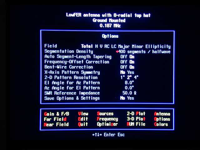
The picture below is a camera shot of the AO main menu screen with the "options" dialog box opened. NF has an identical main menu and options screen, except that you can't select the "2D Plot", "3D Plot" or "Optimize" features. For LowFER antenna modeling, I typically set the segmentation density to a fairly high value like the 400 segments per halfwave shown in the screenshot, because the individual wires making up the antenna are such a small fraction of a wavelength long. The elevation angle for the azimuth pattern is set to 8 degrees, which is probably close to the maximum "takeoff angle" for LF sky-wave propagation. Even though the NF software doesn't have a pattern plotting function, it is important to specify the correct elevation angle for the azimuth plot because this will affect the number shown for the gain. If you set the elevation angle to zero, the reported gain will be some extremely low number, because the gain calculation is made for very great distances from the antenna where the signal level at the (lossy) earth's surface has decayed essentially to zero. The ground losses can be set to zero in AO or NF by using the DOS command SET GND=0 prior to running the program. This will keep the radiation from "disappearing" at very low angles, but it's not a realistic simulation. Skywave propagation is not considered in the MININEC calculations; you have to know something about propagation at the frequency of interest in order to decide what takeoff angle is optimum. There is, however, a near-field option which will be discussed later.
AO main menu with Options dialog box opened
Pressing the letter "V" on the keyboard will bring up the "View" option, providing a 3-d view of the antenna model as shown below. In this case, the antenna is a LowFER vertical with an 8-radial top hat.It's hard to see in this somewhat fuzzy camera shot, but the individual "segments" that make up the model are identified by colored dots, as are the positions of the source(s) and load(s). While in the view mode, you can rotate the antenna picture to any orientation using the arrow keys, expand or shrink it, save the plot as a black-and-white PCX file, toggle the display of source/segment locations, etc. Pressing alt-h in the view mode brings up a help window with a summary of the option keys.
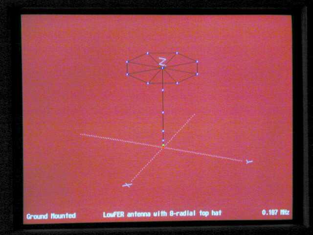
"View" option
From the main menu, pressing "G" will initiate the gain and impedance calculation, resulting in the information that is presented on the screenshot below. Most of the entries are self-explanatory except for the "matrix fill" and "matrix factor" lines. These entries show the time in seconds that was required to do the two calculation steps, in which the interactions between each individual "segment" and every other segment in the antenna are computed. For this example, the times were 0 and 0 seconds on a 233 MHz computer. As mentioned earlier, Beezley's software is fast! At the time I took this picture, I hadn't finalized the value of the loading inductor, so there is still a small reactive term in the impedance. Considering that the antenna reactance without any loading inductance is over 2700 ohms, the value of L is already within about 0.5 per cent of the resonant value, and there is not much point in refining the model any further.
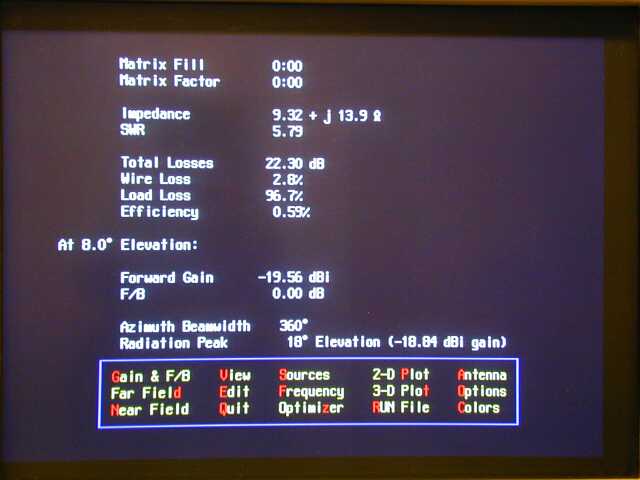
Results of gain and impedance calculation
After a gain computation has been completed, pressing V for "view" will bring up a picture of the antenna with a graphical representation of the currents shown as yellow lines, as in the figure below. Without the top hat, the current distribution in the vertical section of a LowFER antenna would be almost a straight line, with the current dropping to zero at the top. Adding the top hat has made the current much more uniform and has therefore increased the radiation from the antenna. It's difficult to get an exact idea of the currents from the 3-d view, but pressing R while in the main menu brings up the "Run" file. This is a text file that includes the original model information, results of the gain and impedance calculation, and a tabulation of the magnitude and phase of the currents in every "pulse", or segment of the model.
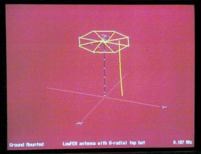
Antenna view with graphical display of current distribution
There is no plot function in the NF software, but this is not much of a disadvantage when modeling LowFER antennas. No matter how you bend, tilt or twist a legal-sized LowFER antenna, its radiation pattern will always have essentially the same shape as that of an infinitesimal vertical monopole over earth. Despite popular myths and claims made for certain antennas, the position of the loading coil and the shape (or even the presence) of the top hat will not change the azimuth pattern or the amount of low-angle radiation. When you're dealing with vertical antennas that are less than 1/100th of a wavelength in size, if you've seen one, you've seem 'em all. The pattern plots below were generated by AO 6.5 for the antenna shown in the view above. Any other LowFER vertical will have the same pattern shape; however the gain figures corresponding to the outer rings of the patterns will vary considerably depending on the efficiency.
The apparent pattern null at zero elevation angle is not a property
of the antenna but of the propagation over lossy ground, as discussed earlier.
Setting the ground losses to zero would eliminate the null and make the
pattern look more like the top half of a vertical dipole pattern in free
space.
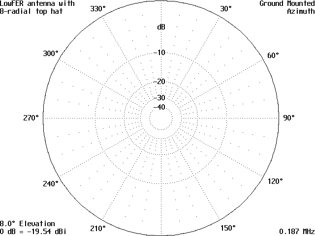
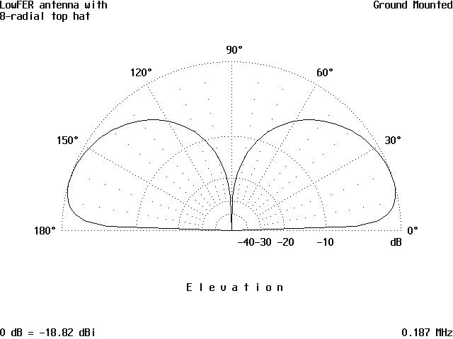
Azimuth and elevation patterns of typical LowFER vertical antennas
In the case of a small loop, the azimuth and elevation patterns will of course be considerably different from those of a vertical, as shown below for a 15 meter square loop made of 1" diameter copper tubing. Here again, it makes essentially no difference in the shape of the pattern whether the loop is 1 meter or 15 meters square; if it is 1 meter or 15 meters above ground, and whether it is fed on the top, bottom or side. Of course the size of the loop drastically affects the gain. The 15-meter loop actually looks pretty good in terms of gain at 8 degrees; less than 1 dB down from the top-hatted vertical. However, in the case of the vertical I included a loading coil Q of 700 and an estimated ground resistance of 5 ohms in the model. The 15 meter loop model assumed no losses from ground proximity (perfectly conducting ground) and no losses in the capacitor (approximately 0.01 uF) needed to tune the loop to resonance. In practice the ground losses and and other factors would cause a significant increase in the loop resistance beyond the 0.085 ohms which the model predicts for the RF losses in the copper tubing alone.
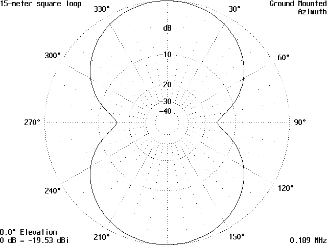
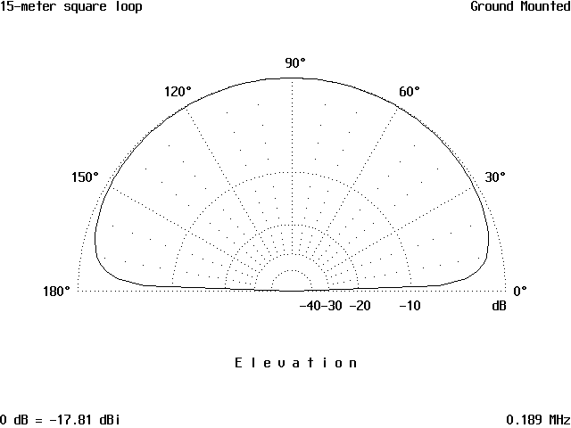
Radiation patterns of small loop above ground
Although NF won't do far-field pattern plots that take ground reflections into account, pressing the "N" key from the main menu will activate the near-field option. You can specify at what points you want the calculation performed, and whether you want to see the electric or magnetic field. NF (or AO) will compute the X, Y and Z components of the field at each specified location (assuming perfect ground) and write the results to the RUN file. I haven't made much use of this feature, but it provides a way of checking your antenna model for accuracy against actual field strength measurements.
I won't go into a great deal of detail on the various modeling options in AO; there is a multi-page documentation file included with the nf.zip file that explains it all. AO and NF use a plain text file to enter the model parameters. Any word processor or text editor that is capable of saving files in ASCII text format can be used to define the model, but there are rigid rules on what goes where. Fortunately the nf.zip file also includes a large library of predefined models for many kinds of antennas which can be used as starting points for a design. I have also packed a number of LowFER antenna designs into a zip file which is available for downloading below. Here is an example of one of the library files included in nf.zip. This specifies a LowFER vertical consisting of a single #12 copper wire, 50 feet long. The comments after the semicolons are my notes on what each line contains. As with many other software routines, anything that appears on a line after a semicolon is ignored by the program, so you can add comments to help remember what all the numbers mean the next time you use a model. I've also used double spacing between lines for clarity. Extra spaces on a line or extra spaces between lines are ignored.
Lowfer Vertical ;(title of model)
Over Ground ;(location -- over ground; free space, or free space symmetrical)
175 Khz ;(frequency of operation)
1 copper wire, feet ;(number of wires; wire material; units of wire dimensions)
10 0 0 0 0 0 50 #12 ;(number of segments; xyz coordinates of start and end; diameter)
1 source ;(number of sources)
Wire 1, end1 ;(location of source)
1 load ;(number of loads)
Wire 1, end1 8403 uH 30 ohms ;(location and value of load)
Beezley's remarks at this point in the antenna file have been deleted for brevity.
The first line is the title, which can be fairly long (but probably not over one line -- I've never tried it). Next is a line that tells the model whether the antenna is over ground or in free space. There is also a "free space symmetrical" condition that will speed the computation and/or allow twice as many segments in the model. We won't worry about the free-space stuff unless someone decides to take a LowFER station along on the Space Shuttle. After that comes a line defining the frequency of operation. (The main menu of NF also lets you perform computations at another frequency or over a whole range of frequencies without modifying the model.) Next there is a line with the number of wires, wire material and the dimensional units for the model. If you specify 20 wires, there had better be 20 lines defining the individual wires or the program will bomb. Each wire is defined by specifying the minimum number of segments you want to use in the modeling process. I usually put a "1" at the beginning of the line and let the software add as many segments as necessary to meet the "segmentation density" that I specify under "options" in the main menu. After the number of segments, it is necessary to specify the x,y and z coordinates of the beginning and end of the wire. Entering six numbers in a row with single spaces between them is adequate for the software to understand, but I always add some spaces to make the file more readable. At the end of the line is the diameter of the wire. Wire material and dimensions can be overridden for any wire in the model by putting in the units rather than simply a number. For example, if I change the line in the model above to read:
10 0 0 0 0 0 15m 1" 6061-T6
it will make the wire 15 meters long,1 inch in diameter, of aluminum alloy material. The original line already had an override in it, which specified the wire as #12, meaning number 12 AWG.
After all the wires (in this case there's only one) are defined, the number of sources and loads and their locations are specified. In AO and NF, source and load positions can be specified only at the center or at the ends of a wire. Since sources and loads must be located at a segment boundary, it will not always be possible for the software to put a source or load at the exact center of the wire, and when you bring up the model it will alert you with a message to that effect. As seen in this example, a source and load can be placed at the same location. Two sources or two loads can not be at the same position; however complex loads are permitted. In this example, the loading coil is specified as having an inductance of 8403 uH and a series resistance of 30 ohms. It's also possible to specify the coil Q rather than putting in a fixed resistance; for example by saying 8403 uH Q=300.
One nice feature of AO and NF is the ability to use symbolic dimensions. In other words, dimensions that are repeated often in the model can be specified by symbols that are defined just before the list of wires. If you want to alter a given dimension, for example the overall height of an antenna with a multiple-wire top hat, you can go into the model and change one number, rather than a whole array of numbers. In the example below, I've used symbolic dimensions to specify a LowFER vertical that is very similar to the model above. However, another wire has been added, and the dimensions of the antenna have been defined symbolically so that it is easy to go into the model and vary the overall height or "slide" the loading coil up or down to see the effect on the amount of inductance required and on the efficiency of the antenna. I've also added symbols for the estimated ground resistance (which I've placed along with the source at the very bottom of the antenna) and for the loading coil inductance. When using the AO software with its automatic optimization feature, it should be possible to let the program calculate the value of L required for resonance, by telling it to optimize L for lowest SWR or to mimimize the imaginary part of the impedance. However, I've found that the optimization program sometimes "gives up" after a few iterations unless the inductor was close to the required value to start with. That's similar to the experience of trying to tune a real-life LowFER antenna without some advance knowledge of the proper inductance value. Small changes in the inductance will produce almost no observable change in the field strength or antenna current when the system is far from resonance. I've found that the fastest "optimization" method is to observe the amount of reactance that AO or NF predicts for the antenna, and then use a hand calculator to determine how much inductance needs to be added if the reactance is negative, or subtracted if the reactance is positive.
Lowfer Vertical with
symbolic dimensions and variable loading coil position
Over Ground
175 Khz
2 copper wires, feet
HL = 1
; height of loading coil above ground
HT = 50
; overall height of antenna
1 0 0 0
0 0 HL #12 ; wire from source to "bottom" of loading
coil
1 0 0 HL
0 0 HT #12 ; wire from "top" of loading coil to top of
antenna
1 source
Wire 1, end1
2 loads
RG = 5
L = 8500
Wire 1, end1 RG ohms
Wire 1, end2 L
uH Q=300
In this simple example, symbolic dimensions are not much of a time saver. However, it would make a big difference in the amount of time needed to modify, for example, the geometry of an antenna with eight top radials and eight skirt wires.
One other difference between this model and Beezley's simple vertical is that I've reduced the minimum number of segments in each wire to 1. If either wire is left with the minimum number of segments set to 10, there will be an error condition when the loading coil is located closer than about five feet to the top or the bottom of the antenna, because segments shorter than 0.0001 wavelength are present.
LFMODELS.ZIP contains a number of models that I've developed for use with AO or NF. The models are somewhat generic, in that each one uses symbolic dimensions. To use the files, unzip them to the same directory in which you have placed AO.EXE or NF.EXE. When you start the program or bring up the "antennas" list from the main menu, all of the models should appear on the list. In order to avoid cluttering the general ham antenna list with a bunch of LowFER antennas or vice versa, you can put the LowFER files in a separate directory and go to "OTHER" in the list of antennas; then type in the path to the proper directory. There's an easier method for keeping the files separate in this day of huge hard drives -- put the LowFER antennas in their own directory and store an extra copy of NF.EXE and its built in text editor ED.EXE in the same directory. It's only 133 kB total; a drop in the bucket by Windoze standards. Here is a list of the files contained in LF-MODEL.ZIP, along with a brief description of each model.
HAT8.ANT:
This LowFER vertical has a top hat with
8 horizontal radials and a skirt wire connecting the outer ends of the
radials. The "conservative" definition of a legal Part 15 LowFER antenna
is used, meaning that the sum of the height (H) of the antenna plus the
length (R) of the radials is constrained to a value called Hmax. You can
customize the model by changing the value of Hmax and R, and/or by redefining
the top hat height to be a fixed value rather than letting it "float" at
Hmax - R. The position of the loading coil can be varied by changing
the parameter HL. Similarly, the values
for the loading coil inductance L can be changed to achieve resonance,
and the assumed ground loss RG and the coil Q can be redefined as needed
to bring them closer to measured values. I have not tried using symbolic
dimensions for the diameters of the various wires used in the antenna,
but it's easy to change them in a word processor application by using a
search and replace operation -- for example to replace all occurrences
of #8 with #14. When using a text editor other than the one supplied with
AO and NF, be sure to save the file as a plain text file with a .ANT extension;
otherwise the modeling software will not recognize it.
HAT3.ANT, HAT4.ANT, HAT6.ANT, HAT12.ANT:
Same as HAT8.ANT but with 3, 4, 6 and 12 top hat radials, respectively.
HAT3NS.ANT, HAT4NS.ANT, HAT6NS.ANT, HAT12NS.ANT:
Like HAT3 through HAT12, except that the skirt wires have been removed.
FLT-TOP1.ANT, FLT-TOP2.ANT, FLT-TOP3.ANT, FLT-TOP4.ANT:
FLT-TOP2 through FLT-TOP4 are "flat top" antennas with 3 horizontal spreaders (one in the middle, one at each end), and 2, 3 or 4 longitudinal wires, respectively. FLT-TOP1 is a simple T antenna. These antennas are of the type that would be suspended between two supports.
HAT3SL.ANT:
This represents an antenna where the guy wires provide the top hat function. In this model the length of the top radials is not included in the overall height allowance. If it had been, the gain would be considerably lower. However, why not let the top radials slope UP instead of down? That would improve the gain considerably, while staying "legal" according to the conservative definition of antenna height. The model allows you to do this by setting a positive value for the angle A1 rather than a negative angle. Building it might be a little tricky, though.
15-MLOOP.ANT
A simple square loop made of copper tubing.
LEK.ANT:
This carries the idea of the upward-sloping radials a step further by using 4 radials (in this case called "downleads"). The "skirt" is a rectangular top hat, formed by two aluminum spreaders connected by two wires. The dimensions given are approximately those of my "LEK" LowFER beacon. LEK's antenna is suspended above the roof of a metal building, and if the height of the building were taken into account in the model, it would further improve the predicted gain.
BEAMHAT.ANT AND BEAMHAT1.ANT:
Using a conventional free-standing antenna tower, it is difficult to insulate the base from ground and still provide a mechanically rugged structure. Shunt feeding is sometimes used on HF and even on MF, but it becomes very difficult to achieve an efficient shunt feeding arrangement for a LowFER antenna using a grounded tower. Fortunately the models show that it doesn't make much difference where you place the source in the vertical portion of a typical top-hatted antenna. So what if you leave the tower base grounded, but insulate the top hat from the tower and feed it with a transmission line running from the ground up to the top hat? It should work, although the shunt capacity between the tower and feed line will cause a significant reduction in efficiency if the loading coil is located near the bottom end of the feed line. Coil position is not critical if a large top hat is used, which means that you can put the loading coil just under the top hat and greatly reduce the losses from the shunt capacitance. Bruce, W0BK uses this scheme for his "BK" beacon and it works very well. At least, the antenna has stayed up a lot longer than any previous version. There's a picture of the BK installation under "Listening for LowFERs, Part 2" on this web site. A 40-foot grounded aluminum tower with a ham HF triband beam and 2-meter vertical on the top doubles as the LowFER transmitting antenna. There is an insulating sleeve between the metal mast and the rotator, and an insulating bushing between the mast and the tower. The main loading coil is located on a standoff at the top of the tower, and a smaller loading coil in Bruce's "shack" is used for fine tuning. It is necessary to isolate the feeds for the triband beam and 2-meter vertical when the LowFER beacon is running. This is accomplished with latching vacuum relays for the HF feedline and with a homebrew isolation transformer on the 2-meter feedline.
BEAMHAT is a model that represents the BK installation (except that it assumes a lower ground loss than Bruce or most other LowFERs can achieve), with the feed line running down to the ground. The shunt capacitance between the mast and tower is included in the model, and it has a significant effect on efficiency. BEAMHAT1 is a more idealized model, with the "source" at the top of the tower and no shunt capacitance. This might approximate the situation where a totally insulating mast is used to support the beam, and a low-loss coax feed running up the tower supplies the RF from the transmitter.
2LF.ANT and 2LF-1FD.ANT:
Under the Part 15 rules, home-brewers can build up to five "devices". Nothing in the rules specifically prohibits running all of them at once, on the same frequency, or even with some advantageous phase relationship. Now, all that might be stretching the rules a bit, but it's interesting to ponder what would happen with two or more identical LowFER beacons in very close proximity. The file 2LF-ANT is simply two of the HAT8 antennas located 40 feet apart and fed in phase from two separate sources. It looks like the gain is almost three dB better than that of a single antenna and the pattern is still essentially omnidirectional. If two separate 1-watt transmitters were used, there would be another doubling of power, resulting in a 6 dB overall improvement in received signal strength. Is the 3 dB antenna gain improvement real, or are we kidding ourselves by assuming that the ground losses for each antenna remain the same as they were for a single antenna? Antenna 2LF-1FD has the same two HAT8 antennas, except that they are connected by a single feed wire running between their bases, and driven by a single source. Now the gain improvement is only on the order of 1 dB. But in this case all the current is flowing through the same ground resistor. Is that fair? Going back to the two antennas with separate sources, they can be separated by 400 feet and there is a hardly noticeable "bulge" in the omnidirectional pattern. The gain is still around 3 db over a single antenna, and it would seem that with this amount of separation the ground losses would be independent. What's the answer? Beats the heck outa me...
CFA.ANT
If all the claims made for the crossed-field antenna are true, eventually all LowFERs will be using them. This file is my attempt to model a 75-meter version that appeared in the Antennex on-line magazine. Proponents of CFAs will argue that existing modeling software is inadequate to handle the special properties of the antenna, and skeptics will say that the apparent successes with a few commercial CFAs in Egypt are due to something other than the CFA structure itself. My modeling results say that the antenna sucks. Not that I have blind faith in MININEC, but I am sure going to wait for more design details and confirming experimental data before building a full-scale LowFER CFA (or even the 75 meter version).
Design Comparisons Using Modeling Results
Here are two examples of how the modeling results can be used to see the effects of changing the antenna design. In the first example, the sum of the antenna height and top hat radius is constrained to 49.2 feet, and we want to see what happens as the top hat size is increased. As the figure below shows, the optimum top hat radius would be between 15 and 20 feet if the ground resistance were extremely low. As the ground resistance increases, the optimum shifts toward a taller antenna with a smaller top hat. These results were obtained by running the HAT8.ANT model with two different assumptions for ground resistance and with varying top hat radial lengths. The reactance of the antenna changes considerably as the radial length is varied, and it is necessary to change the loading coil inductance to achieve resonance. AO can "optimize" the loading coil automatically, but with NF it takes some cut and try. The figure below was generated by writing down the modeling results, then entering them into a Microsoft Works spreadsheet and creating a "chart".
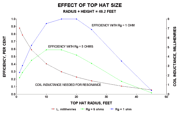
Modeling results obtained on HAT8.ANT at 187 kHz; coil Q = 700
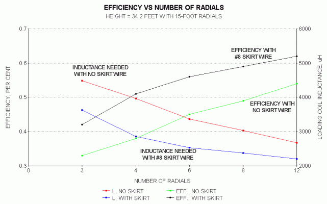
Another good use for the modeling software is to play "what if" games with different numbers of radials to see if the improvement in efficiency is worth the additional challenges in getting the antenna into the air and keeping it there. As an example I ran the HAT3, HAT4, HAT6, HAT8 and HAT12 models, with and without skirt wires, all with 15-foot radials, coil Q = 700 and an assumed ground loss of 5 ohms. The resulting efficiencies and required loading coil inductances are shown below. Once you get beyond four radials, the improvement in efficiency begins to taper off. Also, adding a skirt wire usually does more good than doubling the number of radials.
As with any software, the "garbage in,
garbage out" rule applies to antenna modeling. I don't place a lot of faith
in absolute gain or efficiency numbers for LowFER antennas, because there
is a huge uncertainty in the losses from the ground system and surrounding
objects. Nevertheless, modeling is useful for comparing designs and
to get a better "feel" for how different antennas perform. The best way
to become familiar with antenna modeling software is to download some or
all of the demo/freeware versions available, play with a few models and
see what they do. Have fun!